The concept of unit economics (UE) is quite often discussed amongst founders and investors in the early stage ecosystem. In this article we will present our approach to UE which goes hand in hand with our previously published quantitative approach to product-market fit (PMF) to form the backbone of how we think about evaluating businesses. The aforementioned framework for PMF is focussed on empirically quantifying an existing pattern of interaction between a product and its customers including aspects of growth, lifetime value and concentration. In contrast, the framework presented here for UE focuses on what it costs to generate an observed pattern of PMF with a similar focus on empirical observation. In this article we will present our high-level framework for understanding and visualizing UE for a variety of different businesses as well as show several hopefully illustrative and interesting examples.
When we think about unit economics we are primarily thinking about the following quantity:
gm*LTV – CAC
The three quantities in the above equation are meant to be somewhat impressionistic. From an analyst’s point of view there are choices with regards to what to count in gross margin, CAC and LTV (lifetime value).
To explain the quantities, consider the example of a prototypical SaaS company that sells some software to business customers. In that case gross margin is usually fairly high – in the 80% range. LTV here means empirically observed LTV_n or realized cumulative revenue collected after n months. CAC means all sales and marketing costs needed to acquire and onboard the customer. The salient question that we start with is “how long does it take to get paid back” or, analytically, for what value of n does gm*LTV_n = CAC. This leads one to a payback of n months and the rule of thumb for most venture investors is to consider n<6 months to be great and n>2 years to be not so great and everything in between to be the range of normal. From an investor’s point of view, shorter paybacks translate to leverage on the invested dollar because capital spent on S&M can be recycled faster when paybacks are short. Note that this approach doesn’t use extrapolated LTV. Oftentimes people will compute full LTV using some formula involving imputed parameters (see discussion here). We don’t use that because we’d rather not assume things about the long tail of customer lifetime and instead focus on what has actually transpired. As a result, we tend not to look at quantities such as LTV:CAC because it includes these often spurious extrapolations. Instead, we tend to focus on gm*LTV_n – CAC which we refer to as the “unit (or contribution) margin after n-months”.
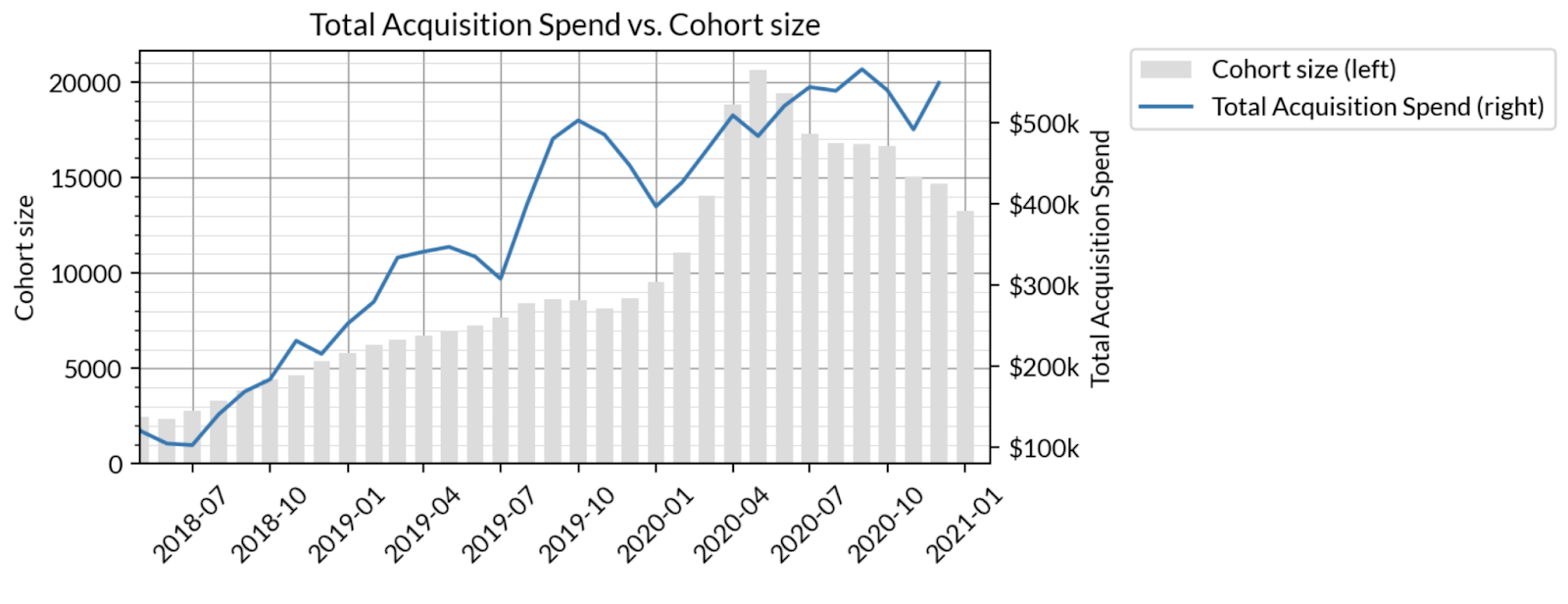
Next up we’ll show how we visualize unit economics. The following graphs reflect artificially generated data that are for the sake of illustration. First up we look at how total acquisition spend has trended and what the resulting cohort sizes were. The blue line in the graph below shows monthly acquisition spend steadily ramping in 2019 from $200k/month up to a current level around $500k/month. The bars show the resulting cohort sizes as being 5k-10k new customers per month before stepping up to 15,000 customers per month starting in mid-2020. Dividing total acquisition spend by cohort sizes gives us a rough estimate for per-unit acquisition cost (which we show on a different graph below) and helps to set the context in terms of the high level growth and spend.
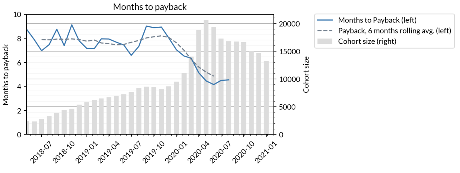
The next chart that we look at is the historical payback chart. Here we see that cohorts in 2018 and H1 2019 were stable at 8 months before falling in early 2020. Note that this is in the context of the previous graph which suggests that the payback increase in late 2019 was commensurate with an increase in spend. The decrease in CAC in early 2020 was at the same level of spend and perhaps is reflecting some 2020 specific phenomena such as the pandemic.
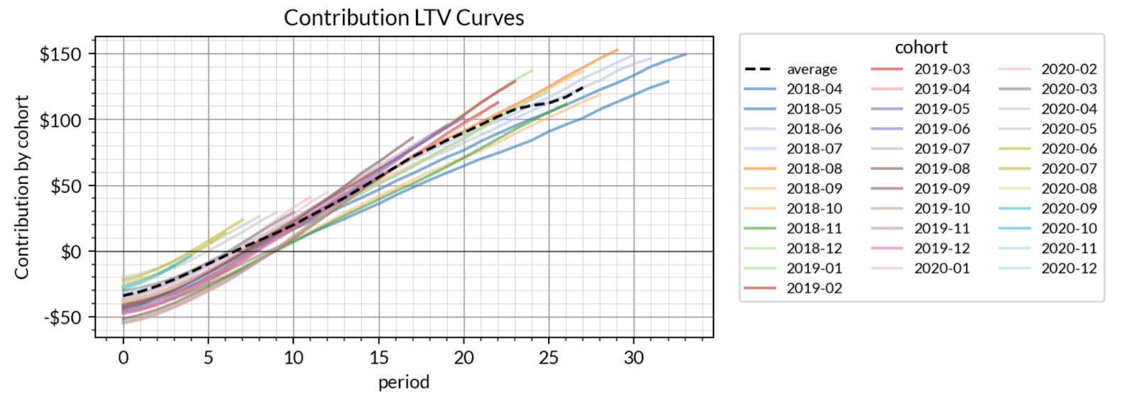
With that context, we now dig into the supporting graphs that inform the payback graph. First up we look at the contribution margin LTV curves. These can be thought of as empirically observed gm*LTV_n – CAC for every single cohort that has come through the business. For those familiar with our prior writing, the LTV curves on their own just represent cumulative revenue collected per customer in each cohort. This graph modifies that by first multiplying the revenue collected by the gross margin and then subtracting the CAC observed for that cohort. By looking at the y-axis you can see that CAC has ranged between $20 and $55 although it’s hard to see the time dependence of that range. When a single cohort’s gm*LTV curve passes the y=$0 line that represents breaking even on the cohort. The dotted line here is the (weighted) average curve which suggests breakeven of 6-7 months. As with regular LTV curves, the value of this visualization is to see the shape of the LTV curves. When LTV curves bend upwards and are superlinear then payback is less sensitive to CAC. In contrast, when LTV curves bend down and are sub-linear then payback can be quite sensitive to CAC as a shift up or down of the gm*LTV curve can make the intercept occur at wildly varying values of n. At some level this is why superlinear LTV curves are preferred – they imply more predictable payback dynamics. Superlinear LTVs are also more likely to render payback times “scale invariant” in the sense described later.
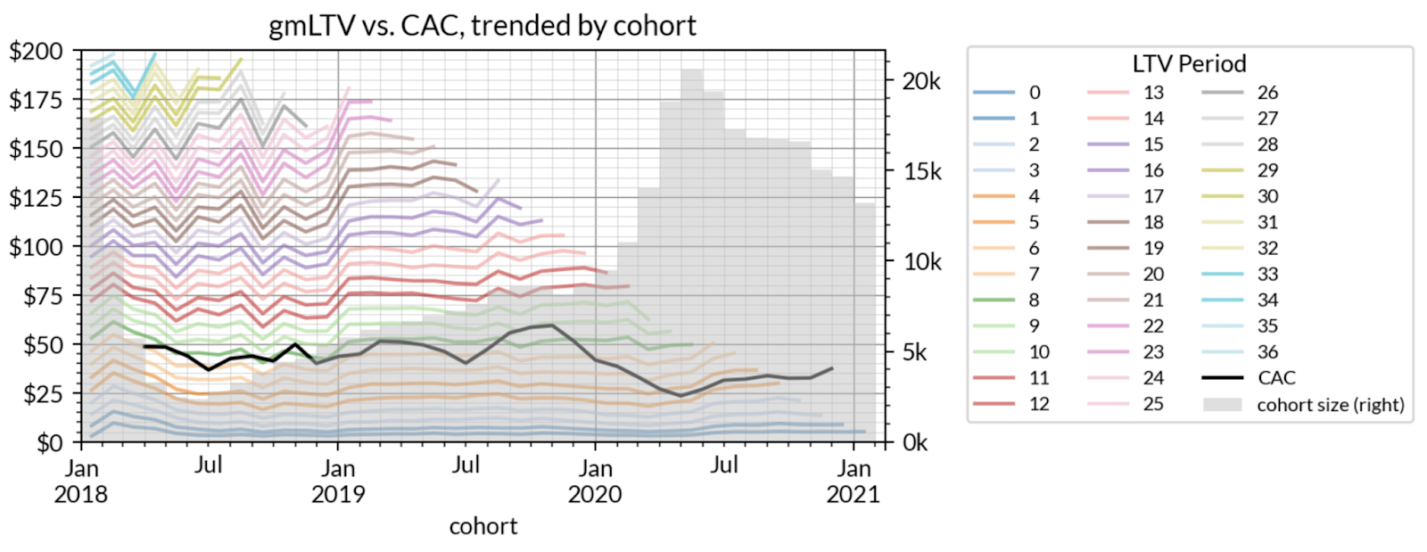
The next visualization is a UE modification of the LTV Trends graph presented in our original article about Quantitative Product-Market Fit. Recall that in that graph we can see specifically how LTV_n has trended as cohorts have gotten larger or smaller at a fixed time horizon of n months. In the unit economic modification of that graph below we show gm*LTV_n for various values of n with the cohort sizes in the grey bars and with the CAC overlay. For cohorts whose gm*LTV is above CAC we know that they have empirically paid back. In this graph the trend of CAC is more clear. In this case we can see that the early 2018 cohorts paid back in ~7 months which increased briefly in the 9+month range in late 2019 while, then down to 4-5 months by May 2020. Although LTVs increased slightly over this time, the main lever here was an increase in marketing efficiency. Just like with the regular LTV trend graph, this graph makes the trend behavior clearer while sacrificing the shape of the LTV curve which is not really obvious in this graph. Hence we look at both when thinking about paybacks. As should be fairly obvious, the crossing of the LTV_n contour lines over CAC determines the payback for that cohort and the payback graph up above follows from those crossing points.
The above four graphs are the main ones we look at to think about unit economics at Tribe. As you can see it’s a fairly natural extension of the Quantitative PMF framework that we have written about before. In some sense the PMF metrics merely indicate whether or not the product is satisfying customers (i.e. generating some PMF) and leaves aside whether or not the business can generate that pattern of PMF while generating a profit. By focusing on the quantity gm*LTV – CAC we can tease out this question of profitability while retaining our flexible thinking on LTV that our quantitative approach to PMF provides.
Turning the Income Statement Sideways: How We Think about Scale Invariance
Now that we have the basic picture outlined we will delve into some of the nuances. The first nuance is how exactly one should interpret gross margin and CAC in the expression gm*LTV – CAC. The answer comes from the concept of “scale invariance”.
From an analytical perspective, our overarching goal of investigating unit economics in the first place is to find a parameter that is robust to scale with the thinking that if the company raises and deploys capital, it is effectively buying more units and the investor hopes that quantities like “payback” stay roughly constant as that capital is deployed and costs ramp up. In order to achieve this, the analytical exercise is to categorize costs into those that will scale with the number of units being acquired vs. those that (hopefully) will not. For example, sales team salaries and onboarding costs are usually thought to scale with the number of units, hence is included in CAC. In contrast, we usually think of the software engineering team as not scaling and hence the cost to pay engineers is not usually included in the UE quantities (although sales engineers are a clear exception to this rule). Similarly, there are situations where a company has to pay for something to deliver the service so the cost should be a COGS but it doesn’t actually scale with the business and so shouldn’t be in the gross margin above (think of paying some flat annual fee for access to some shared infrastructure). One way to think about this is the delta between “gross margin” and “contribution margin”. Gross margin is a concept that accountants use to comply with GAAP requirements whereas contribution margin is a concept that is primarily used by business operators who want to understand their business separate from what accounting standards may suggest. At some level, the act of choosing parameters is the “art” part of the exercise whereas the graphs and analytical manipulations described above are the “science” part. As analysts and students of how businesses grow and scale, we believe that it takes both to create a complete understanding of the relevant dynamics in any given situation.
We also like to think about this approach as “turning the income statement sideways”. When you think of traditional financial statement analysis, the focus is on quarter to quarter (or month to month) revenue and how costs and margin have emerged on a calendar time basis. Calendar based costs are important to consider because if you do it wrong you will simply run out of money. However, technology has enabled us to think about scaling businesses by factors of 10x, 100x, 1,000x and in that case it seems prudent to worry less about the calendar driven profitability and to instead focus on unit driven profitability. While the income statement makes the cash flow more manifest, it does so at the expense of obfuscating the economics over the lifetime of customers which is more clearly laid out in a unit economic framework. Instead of thinking about costs one calendar quarter at a time, unit economics thinks of it one unit at a time regardless of the speed at which the units are acquired – hence “turning the income statement sideways”.
For CAC, we usually group all of sales, marketing, partnerships, onboarding etc. into this quantity on a first pass. However, it’s important to recognize that at some level these don’t all scale the same way. In particular, marketing headcount tends to scale differently from digital marketing budget (think SEO, performance marketing, etc.). Also, partnerships are largely designed with the specific goal of generating non-linear outcomes whereby adding N more folks to partnerships doesn’t generate a proportional amount of revenue. So we often exclude these costs from CAC depending on the circumstance.
Another thing that can sometimes be teased out of the above graphs is how CAC shifts as overall marketing spend moves around. This is often a signal of market depth. When a market is very deep then CAC can stay roughly constant even if you are scaling acquisition spend by multiples. In contrast, when a market is less deep, CAC will often deteriorate as acquisition spend scales.
So with that, we conclude with the main articulation of how we think of UE at Tribe. For the rest of this paper we will walk through some examples. While we won’t necessarily have all the graphs above for each example, we’ll walk through the figurative logic and some back-of-the-envelope calculations to estimate paybacks and discuss what it tells us about the business. After that there is a long FAQ section and, of course, feel free to reach out any time with feedback or questions to jonathan@tribecap.co.
Example: MagicMoneyCo
MagicMoneyCo is a toy example that we often use to illustrate core concepts. MagicMoneyCo is a company that consists of one employee, the founder, standing on the corner selling $1 bills for 90 cents. If one were to run the Quantitative PMF approach on MagicMoneyCo it’s pretty clear that it would be amazing. Growth accounting would show lots of expansion, low churn. Cohorts would all be super linear in LTV and would have very good customer retention and dollar retention. From a PMF pov, MagicMoneyCo would have very clear signs of strong PMF.
However, as should be obvious, it would be a terrible business because it would not be possible to generate the observed pattern of pmf while also generating a profit. Gross margin is -10% so gm*LTV would start at $0 and then slope to negative infinity. While CAC would be zero, it’s fairly clear that payback would never occur.
While MagicMoneyCo seems like a silly example, early stage companies sometimes look like MagicMoneyCo when they are nascent. Gross margins might be negative now but if they scale to some size or sign such and such partnership, gm might go positive. Just because a company looks like MagicMoneyCo at year 1 doesn’t mean it can’t go on to be a massive company. There certainly exist investors (including Tribe on occasion) who will finance the interim while the company tries to find margin and sometimes they can go for a very long time indeed.
Example: Pitfalls in the seed stage
While most of the discussion here focuses on later stage companies, it’s worth describing some of the takeaways that are specific for earlier seed stage companies.
One common thing that we see in the early stage are situations where markets are not yet developed enough for a given product. This often shows itself in being just too hard to sell the product which leads to both high CAC as well as low pricing power which turns into low LTV thus leading to very long paybacks. Long paybacks are not terrible in and of themselves, but it means that you will have to rely on investors to subsidize growth instead of being able to reinvest cash flows from unit profits to drive growth.
Another thing that we see is lack of clarity around what the “unit” is. There are often many equally valid ways to think about unit economics but we tend to focus on the unit that reflects CAC. This nuance often plays out in food oriented companies (delivery, production, supply chain, etc.). Many of these companies have non-trivial COGS so even making a single delivery profitable is a challenge and so a lot of time is spent articulating UE from the point of view of a single meal delivery. While that is important, it doesn’t help to shed light on *growth* which ends up being driven by S&M and CAC considerations. In these cases we will always try to estimate out the UE on the customer basis as opposed to the per-meal basis so that we can get a better handle on what will happen as capital is deployed towards S&M.
Example: Slack via public filings
Their 4Q21 materials suggest that they net added 14k paid customers in the quarter. $123M in sales and marketing. Assuming that they don’t have a lot of logo churn in the quarter would suggest CAC of ~$9k. Slack is right around $1b of ARR across 156k paid customers implying ARR/customer of $6.4k. They also report net dollar retention of 123% which implies that the LTV curve is fairly superlinear. Given that we’re just roughly estimating, we will ignore that nuance and will assume LTV12~$6.4k. This is a pretty bullish assumption because superlinear LTV means that the revenue is mostly in the later part of customer lifetime and thus the overall ARR/customer figure is probably much higher than LTV12 but we’re not aiming for precision here as much as an illustrative example. Being a saas company means gross margin is pretty straightforward at 87%. And so, gm*LTV_N – CAC is roughly 87%*N*$6.4k – $9k implying a payback of about 19 months.
This calculation is averaged across their entire customer base which has non-trivial concentration. Slack has a big free tier with small customers paying $80/year all the way up to very large enterprise customers paying hundreds of thousands of dollars per year. The UE dynamics are very different in the different ends of the spectrum – at the small end it’s about leveraging upgrades from free to paid and on the large end it’s an enterprise sales motion. The averaged values in the above estimate correspond to teams of size 50-100 which is reasonable as an average but it is certainly quite different from the small team use case and the large enterprise use case.
The folks at Theta Equity did a far more in-depth treatment of Slack at their IPO here. They ended up with a 3 year payback largely due to the superlinear shape of the LTV that I mentioned above.
Example: StitchFix via public filings
StitchFix can be estimated based on their investor relations materials. On the LTV side, credit card panels suggest LTV12 ~$630. They also report 43% gross margin implying a gm*LTV12 ~ $270. Contribution margin is probably a better measure (as it would include the stylists etc) here but we’ll stick with this for simplicity.
CAC is a bit trickier. These numbers are obtained from their quarterly report for the period ending Jan 30, 2021. They report $42M of ad spend and $257M of total SG&A respectively per quarter. Their shareholder letter indicates 3.9m active clients (where active is trailing 52 week active) and that this figure had net growth of 110k q/q. Growth accounting can be roughly inferred from credit-card panels which suggest that net growth is ~⅓ of the magnitude of gross new clients so we expect new clients in the quarter to be ~300k. That is, we believe that their acquisition activities added 300k clients and they subsequently lost 200k clients for net addition of ~100k.
This would imply an ads-only CAC of ~$42m/300k ~ $140. If you include all of SG&A then CAC is more like $257m/300k ~ $856. And so depending on how you interpret CAC, payback is between 7 months and 36 months. This is a fairly wide range but it at least gets us to the ballpark. Now SG&A for SFIX includes pretty much everything from stylists, engineers, fulfillment center ops, etc. It’s pretty clear that counting all of SG&A in CAC is not appropriate, but at least we see that at the very worst paybacks are 36 months. A better estimate would probably put stylists into COGS (i.e. gross margin) and exclude engineers from the mix. No doubt there is some internal team at SFIX that watches this in far more granular detail than we are presenting here.
Note other folks have estimated SFIX CAC before (see here and here) yielding a similar range and with most recent estimates in the $700+ range. Indeed, an increasing CAC would suggest that they are running into market saturation (or competition) which can be understood as starting to hit the limits of scale invariance hence UE dynamics deteriorating. Once again, the goal here is not to be precise, but rather to illustrate how the pieces conceptually fit together.
Other things to notice here, the difference between gross and contribution margin is non-trivial in SFIX because of shipping, warehouses and stylists. Figuring out how those should apply to the “gross margin” in the UE calculation requires another level of detail that is likely not possible with only public data.
Example: GTV Based Businesses – Square
Square is a payments business that sells to SMBs, startups and larger enterprises. Let’s say that they acquire a small artisanal cheese merchant who sells at a farmers market. Perhaps that merchant generates $50k in turnover each year on which Square makes ~1% of interchange and fees. In this case gm*LTV in the first year is something like 1%*$50k ~ $500. For the small artisan cheese seller, sales & marketing looks not unlike straight consumer marketing so it’s not unreasonable to expect ~$500-1k CAC. One should also add the cost of the Square device itself to CAC which is probably in the <$50 at this point.
The take rate in interchange businesses is complicated depending on rails, arrangements with banks, etc. So the gm can be anywhere from very low 0.1% all the way up to over 2%. As should be clear from this discussion, payments business UE are highly sensitive to the margin structuring that extracts net revenue from GTV and it is prudent to make sure that this is clearly articulated when considering GTV based businesses.
Example: Insurance
Insurance companies are somewhat different from normal businesses. They get paid a stream of premiums most of which goes towards paying claims (usually via re-insurers, a fronting carrier, or some other arrangement). Presuming that the insurer is good at handling risk then they will realize a healthy margin on the premium stream. At scale, gm*LTV_n is something like (1-loss ratio)*k*annual_premium. Looking at Lemonade’s S-1 suggests an annual premium is $183 with a loss ratio of ~72% which implies $51 of gross profit in year 1. They seem to suggest a rough CAC of ~$90 which would imply a payback in roughly 2 years.
You can see how various groups within an insuretech work on various pieces of UE. The marketing team aims to lower CAC, the tech-product team aims to increase retention and thus raise LTV, the insurance-product team aims to underwrite better and thus lower loss_ratio. Effectively, every team’s work is reflected in the UE structure.
Example: Asset management
In the modern era there has been a lot of innovation in tech enabled asset managers whether they be robo-advisors or tech-enabled buyout strategies. For the consumer examples, gm*LTV_n is usually something like a take rate on AUM. So if you can acquire $10k in AUM and make 1% per year then gm*LTV_n is something like 80%*1%*10k*n ~$80*n i.e. $80 per year (assuming low churn which is the historical norm in legacy consumer financial services). So presuming you can acquire users for less than $80 you will be paid back in a year. Of course, in the consumer realm, paid acquisition runs up against everybody else trying to market to consumers which usually drives CAC way above this estimate and drives paybacks out into the multiple-years range. Hence, most fintechs believe that they can make more money in the future by tacking on additional high margin services such as loans, etc. Indeed, in fintechs most of the action happens well after the payback period when these additional services can be introduced. Nonetheless, understanding the near-term structure of the payback is important because startups are more likely to fail in the near-term than in the long-term.
It’s interesting to consider the “enterprise” version of this set-up of which private equity/venture capital is an example. In that case, assume you can raise $10m in a fund and collect 2% fee and 20% carry. Also assume that the fund lasts for 10 years and achieves a 2x gross multiple (this is a rather low bar but is actually the median fund according to fund returns data), then gm*LTV over 10 years is something like 10*2%*$10m + 20%*$10m = $4m. If it’s a “European waterfall” then the fees have to be paid back first in which case it’s actually more like $2m. This is over the 10 year life of the fund, so if you amortize over the 10 years and spend $200k to acquire the AUM in the first year then it “pays back” in roughly one year. It turns out that CAC for acquiring AUM in asset management is very widely varying and hard to engineer which is why it’s hard to build investment firms.
Example: Ridesharing As An Example of Marketplaces
For our final example, we’ll talk through ridesharing as an example of a marketplace and how unit economics works in this context. For simplicity we’ll use Uber and will estimate figures from a combination of their annual report from 2019 Q4 (pre-COVID) and from credit card panel data.
In the first pass we consider the rider to be the unit. In that case there is some GTV LTV per rider (turns out to be ~$170 at 12 months according to credit card panels). They also spend a fair bit on rider marketing and promotions which drives some CAC_rider. The tricky nuanced piece here is what to use as the effective margin. Clearly gm should include the costs of paying the driver and Uber reported net revenue take per-ride to be 23%. But one should also include the costs to maintain the pool of drivers that are needed to actually generate the GTV. Let’s say that in a given market they need to maintain 10k drivers and that they spend $2m on driver acquisition and promotions during that time (i.e. $200/driver/month) to maintain the driver pool and that this market generates $30m in GTV. Thus for $30m of GTV in this market, there are (100%-23%)*$30m = $23m of costs to the driver and $2m of extra costs to maintain the driver pool and the effective margin here is ($30m-$23m-$2m)/$30m = 17% which is lower than the 23% take rate because it takes into account the costs needed to maintain the supply pool. With this, gm_eff*LTV12 ~ 17%*$170 = $28. Rider CAC is non-trivial because acquiring consumers is expensive, so this payback is probably well over 24 months. Something else to notice here is that if it costs much more than $2m/month to maintain the driver pool then it is possible for the effective margin to be negative. This intuitively makes sense – if it’s too expensive to maintain drivers then the incremental rider will never pay back with the LTV and take rate assumptions above.
Alternatively, you could view the unit as the driver. In that case, LTV is the GTV LTV of a single driver. The effective margin to the company is once again 23% reduced by an amount reflecting the costs to maintain the *rider* pool needed to keep the supply engaged. Taking the same example as above, that $30m of GTV was probably from ~ 375k distinct riders (pre-COVID Uber riders averaged $80 GTV/month) and they probably have to reacquire 20% of them per month at $60 each so there are probably $4m of ongoing costs here. And so the effective margin here should be ($30m – $23m – $4m)/$30m = 10%. For LTV12, Uber in 2019 reported 7b trips from 5m drivers which is 1.4k trips/driver/year. We will make the simplifying assumption that LTV12 is roughly this number (which is almost certainly not the case as there are probably older drivers who are dragging the average up). We then use the fact that average ride value is ~$15 giving us a GTV LTV12 from the driver side of $21k. And so gm_eff*LTV12 ~ 10%*$21k ~ $2k. This is pretty high and you can see why Uber and Lyft are willing to spend a fair bit acquiring and onboarding new drivers. Once again, if the market is such that acquiring drivers is easy but maintaining a demand base is expensive, it is possible to never be paid back on incremental driver CAC.
A third viewpoint would view the unit as the ride transaction itself. This case is somewhat equivalent to opening up an entire market or perhaps buying a company that operates in the local market. In this case, let’s say that the whole market will generate $30m in its first year so LTV12 is $30m. The margin now needs to take into account the costs to maintain both the supply and demand sides which are $2m and $4m respectively from our example above. So the effective margin is ($30m – $23m – $2m – $4m)/$30m = 3%. And so gm_eff*LTV12 ~ 3%*$30m ~ $1m and if you can buy the local operation for $10m then you get paid back in 10 years.
With this example above you can see that depending on the payback structure of each side of the marketplace it may be more beneficial to deploy the marginal dollar to either supply or demand side acquisition. If they are in a market where demand is plentiful but there are lots of credible alternative jobs then CAC on drivers will be much higher and figuring out product features, promotions or partnerships to give a structural advantage to the supply side will have a big effect on lowering CAC. When we look at marketplace opportunities at Tribe a big part of what we try to figure out is how the supply and demand sides will unfold through different unit economic lenses and the generalized analytical framework described here forms the backbone of how we think about those dynamics.
We’re a venture capital firm focused on recognizing and amplifying product-market fit. Reach us at hello@tribecap.co.
FAQ
Q: What about LTV:CAC?
Many companies will quote LTV:CAC where LTV is calculated as an inferred figure based on observed churn early in the lifetime of cohorts. We find this not very useful because we find the inferred LTV to be mostly useless and time horizons arbitrary. All interesting companies have LTV curves that are linear or better and thus the inferred LTV is infinite which is clearly meaningless. Hence why we focus on payback as opposed to LTV:CAC.
That said, there do exist businesses with fairly stable infinite time horizon LTVs – life insurance is a pretty good example. For those types of businesses LTV:CAC might actually be a more well defined concept and may actually be scale invariant. LTV:CAC can also be inferred as return-on-ad-spend in ads driven businesses or perhaps multiple-of-invested-capital in asset management businesses.
Q: What about segmentation?
This is partially covered in the Slack example above, but it should be clear that for companies with highly variable customer contracts, UE can behave very differently in different segments. For example, in B2B SaaS companies there is often a big difference between enterprise contracts vs. self-serve/SMB contracts.
On the SMB side, CAC oftentimes is driven by top-of-funnel marketing or perhaps might include the costs of running a free tier of the business. LTV will be determined by being able to execute expansion while mitigating churn for these customers without spending a lot on customer success. In contrast, on the enterprise side, CAC is driven by enterprise sales which has a very different cost profile. LTV are often very large and complex contract structures can bake in the shape and margin structure for more of the LTV curve. From an investor’s perspective it is often useful to know both the fully blended UE as well as the segmented UE.
Q: Is my payback good/bad?
Rule of thumb for B2B SaaS companies tends to be that paybacks under 6 months are solid while paybacks over 2 years are not so great. Oftentimes the paybacks get longer as the company gets bigger as they are acquiring more marginal customers at that point. That said, this is just a rule of thumb. There are many great companies that have had longer paybacks even from an early stage and, similarly, many companies that have flamed out even with short paybacks.
The best situations are when the product itself generates growth which can render CAC to be extremely low even down to the sub $1 range. This is most often accomplished via some viral growth mechanism. In these situations the problem becomes less about CAC than about how to create revenue LTV without disrupting the product-led growth pattern.
Q: Is faster growth worth more than short paybacks?
The tradeoff between payback and growth is a common one that founders face. Depending on the specific dynamics that a company faces around competitors, macro effects, investor appetite, etc. the tradeoff may favor one direction or the other. We find that the best situations are the ones where we can have a clear quantitative sense of just how paybacks will react if we push to grow by another ~5% per month. It’s our observation that the early stage market for the last several years (as of writing this in mid-2021) has valued top-line growth more than payback and margin structure. While this is the case now, it doesn’t mean that it will always be the case and part of what we try to do with founders is to figure out the right mix of growth and margins given their specific circumstances and objectives.
Q: How do UE/paybacks affect valuations?
In the public equity markets it is usually not possible to get detailed unit economic information. As such, most companies are valued on more macroscopic variables that are easier to observe such as revenue scale, growth, margins, EBITDA, etc. Given that valuations in the early stage have to eventually get comped to public market valuations, we typically find that valuations in the private markets similarly tend to follow these macroscopic variables. That said, UE quantities clearly affect how those macro quantities evolve and interact. Indeed, we view UE and PMF metrics as the two underlying structures that drive the macro growth and operating margin variables and, as such, UE affects valuation indirectly through those quantities.
Q: Why is gross/contribution margin included?
We sometimes see founders present their paybacks on a revenue basis, particularly for pure software companies where gross margin and contribution margin are both quite high and not materially different from each other. The picture changes though when there are non-trivial COGS such as physical goods, payment processing, delivery costs, ongoing operational costs etc. In these cases the guiding principle is scale invariance and excluding these costs from UE thus leaves these scale sensitive costs in the OPEX. In addition, one of the goals of UE is to help us to understand the cash recycling capabilities of the business – short paybacks mean that you can redeploy unit profits to acquire more units. As such, gross/contribution margin has to be included otherwise it will not be a faithful representation of cash flowing back through the customer lifecycle.
Q: What about Growth Accounting?
Growth accounting is a way to quantify the components of top line growth. The cost of that top line growth on a calendar basis is evident in P&L. At some level, the income statement is “how spending S&M relates to driving growth” whereas unit economics is “how spending S&M relates to driving margins”. We view them as fairly different and don’t generally think that growth accounting has much bearing on unit economics. That said, growth accounting is often useful in cleanly articulating new customers vs. other types of customers and hence the customers which were “bought” with the S&M spend.
Q: What about Retention?
Retention shows up in UE via LTV. A low retaining product will generate lower/sub-linear LTVs which will generate the issue mentioned above around sensitive paybacks. Sensitive paybacks are, pretty much by definition, less likely to be scale invariant.
Q: What about 80/20?
It is possible to analyze the distribution of lifetime contribution margin across a cohort of customers. Sometimes when a cohort has good UE and has paid back, this could be driven by one outlier customer driving positive UE offsetting a bunch of UE-negative customers. While this could be true for a single cohort, it’s harder for it to be true for a dozen cohorts. If you have a dozen cohorts that are all UE positive after 6-9 months, then there would have to be some unusual time distribution of whales to make that happen. Possible but unlikely.
Q: What about non-dollar LTVs?
LTV as a concept can apply to non-financial exchanges of value between a product and a customer. For example, one can consider the “posted tweets” LTV of Twitter where LTV_n would be cumulative tweets after k-months. In some sense, one has to believe that an engagement oriented LTV_n has some translation into actual revenue. The reason being that S&M represents actual dollars used to acquire customers and so you have to believe that you’ll get paid back one day. If you don’t believe that the engagement LTV will pay back one day then the business is equivalent to MagicMoneyCo and is probably not interesting.
Q: How is this useful to an operator?
From an operating viewpoint, at some level, it is often useful to think of projects as specifically focusing on some facet of the unit economics equation. For example, Uber might have a driver retention team that is focusing on the LTV of drivers. Or perhaps they have a partnerships team which is fundamentally trying to lower CAC, etc. For teams that work on consumer social products where monetization is left for the future (e.g. early Facebook) one can often still interpret projects through this lens as, for example, retention/engagement projects are fundamentally affecting usage LTV which is related to monetizable LTV in some concrete manner.
Q: My company has great payback. Will you invest?
As with the PMF approach to understanding the structure of demand, unit economics is just one facet of our investment process at Tribe. Having great unit economics (or at least a clear path to great unit economics) is usually an important feature for a potentially great company, but it is by no means sufficient.
Q: This seems more important than the 8-ball. Discuss!
We view the 8-ball as giving a framework that helps us understand any given pattern of PMF but it doesn’t say anything about what it costs to create the pattern or whether or not it is possible to make a margin on it.
Q: Why don’t they teach this in my MBA?
The framing around empirical lifetime value is something that is relatively recent because computing actual LTV requires detailed customer level data and computational technology that has been in widespread use only for the past 10-15 years or so. While the analytical techniques described here are fairly commonly used in modern tech companies, they would have been the absolute cutting edge a generation ago and thus have not had the time to fully diffuse into the academic curriculum.
Q: Can you share an Excel template to compute this?
Really no Excel is needed. To compute and visualize LTV, please refer to A Quantitative Approach to PMF. The modifications necessary to visualize the UE modifications of those graphs are straightforward from there.
Q: “Scale invariance”, what are you, physicists?
The concept of scale invariance has a long and impressive history in physics. The physical systems of interest to physicists are typically simple enough to be well described by some set of equations and principles (in particular, systems described by the principle of least action). There is a whole mathematical formalism called the renormalization group which provides a systematic way to transform quantities in those physical systems as the scale of the system changes. While it would be nice if the interaction of a product with customers were well captured by something like a principle of least action which could, in turn, have some sort of well behaved scale invariant behavior, we have yet to find such universal analytical models that are good descriptions of a wide range of product-customer interaction. If anything, the goal of the investor is to find exactly those companies which may indeed have some scale invariant dynamics because it might be exactly those that we can “model” and safely extrapolate through multiple scales. Indeed, early social networks exhibited some of this behavior. At some level there were some dynamics around engagement and growth in early Facebook and those dynamics turned to be roughly invariant as the user base grew from 10m to 100m to 1b users. This line of thinking is pretty interesting and we continue to ruminate on it but will leave it to the reader to come up with more thoughts.